Tesla Stock Prediction using Web Scraping and Recurrent Neural Networks

Stock Prediction is a versatile and extensive field on its own. With increasingly sophisticated computational capabilities, Stock Prediction is becoming a more and more important application of fields like Machine Learning, Deep Learning and AI.
This project deals with web scraping Tesla stock prices from the Yahoo Finance page, using Beautiful Soup and Selenium, and using Recurrent Neural Networks (particularly LSTMs) to build a Deep Learning model to predict future stock prices.
Importing the necessary libraries:
import os
import tensorflow as tf
import numpy as np
import matplotlib.pyplot as plt
from matplotlib import style
import matplotlib
import pandas as pd
from datetime import datetime
Since this is executed in Google Colab, the Google Drive containing the web-scraped data is contained here.
The code for the webscraping, executed with BeautifulSoup and Selenium, can be found here.
from google.colab import drive
drive.mount('/content/gdrive', force_remount=True)
root_dir = "/content/gdrive/My Drive/"
data_dir=os.path.join(root_dir,"tsla.csv")
Go to this URL in a browser: https://accounts.google.com/o/oauth2/auth?client_id=947318989803-6bn6qk8qdgf4n4g3pfee6491hc0brc4i.apps.googleusercontent.com&redirect_uri=urn%3aietf%3awg%3aoauth%3a2.0%3aoob&response_type=code&scope=email%20https%3a%2f%2fwww.googleapis.com%2fauth%2fdocs.test%20https%3a%2f%2fwww.googleapis.com%2fauth%2fdrive%20https%3a%2f%2fwww.googleapis.com%2fauth%2fdrive.photos.readonly%20https%3a%2f%2fwww.googleapis.com%2fauth%2fpeopleapi.readonly

Enter your authorization code:
··········
Mounted at /content/gdrive
Creating a function to plot Time Series Data:
def plot_series(time, series, format="-", start=0, end=None):
    plt.plot(time[start:end], series[start:end], format)
    plt.xlabel("Time")
    plt.ylabel("Value")
    plt.grid(True)
Reading in the data, using Pandas:
df=pd.read_csv(data_dir)
df
| Unnamed: 0 | Date | Open | High | Low | Close* | Adj Close** | Volume | |
|---|---|---|---|---|---|---|---|---|
| 0 | 0 | Apr 29, 2020 | 790.17 | 803.20 | 783.16 | 800.51 | 800.51 | 15812100 |
| 1 | 1 | Apr 28, 2020 | 795.64 | 805.00 | 756.69 | 769.12 | 769.12 | 15222000 |
| 2 | 2 | Apr 27, 2020 | 737.61 | 799.49 | 735.00 | 798.75 | 798.75 | 20681400 |
| 3 | 3 | Apr 24, 2020 | 710.81 | 730.73 | 698.18 | 725.15 | 725.15 | 13237600 |
| 4 | 4 | Apr 23, 2020 | 727.60 | 734.00 | 703.13 | 705.63 | 705.63 | 13236700 |
| ... | ... | ... | ... | ... | ... | ... | ... | ... |
| 248 | 248 | May 06, 2019 | 250.02 | 258.35 | 248.50 | 255.34 | 255.34 | 10833900 |
| 249 | 249 | May 03, 2019 | 243.86 | 256.61 | 243.49 | 255.03 | 255.03 | 23706800 |
| 250 | 250 | May 02, 2019 | 245.52 | 247.13 | 237.72 | 244.10 | 244.10 | 18159300 |
| 251 | 251 | May 01, 2019 | 238.85 | 240.00 | 231.50 | 234.01 | 234.01 | 10704400 |
| 252 | 252 | Apr 30, 2019 | 242.06 | 244.21 | 237.00 | 238.69 | 238.69 | 9464600 |
253 rows × 8 columns
There’s a year’s worth of stock prices here, from April 30, 2019 to April 29, 2020, with a few days’ data missing.
But first, there is some Data Cleaning that needs to be done:
The columns “Close” and “Adj Close” have additional * symbols which have to be removed:
df.drop(labels="Unnamed: 0", axis=1, inplace=True)
df.rename(columns={"Close*": "Close", "Adj Close**": "Adj Close"},inplace=True)
df
| Date | Open | High | Low | Close | Adj Close | Volume | |
|---|---|---|---|---|---|---|---|
| 0 | Apr 29, 2020 | 790.17 | 803.20 | 783.16 | 800.51 | 800.51 | 15812100 |
| 1 | Apr 28, 2020 | 795.64 | 805.00 | 756.69 | 769.12 | 769.12 | 15222000 |
| 2 | Apr 27, 2020 | 737.61 | 799.49 | 735.00 | 798.75 | 798.75 | 20681400 |
| 3 | Apr 24, 2020 | 710.81 | 730.73 | 698.18 | 725.15 | 725.15 | 13237600 |
| 4 | Apr 23, 2020 | 727.60 | 734.00 | 703.13 | 705.63 | 705.63 | 13236700 |
| ... | ... | ... | ... | ... | ... | ... | ... |
| 248 | May 06, 2019 | 250.02 | 258.35 | 248.50 | 255.34 | 255.34 | 10833900 |
| 249 | May 03, 2019 | 243.86 | 256.61 | 243.49 | 255.03 | 255.03 | 23706800 |
| 250 | May 02, 2019 | 245.52 | 247.13 | 237.72 | 244.10 | 244.10 | 18159300 |
| 251 | May 01, 2019 | 238.85 | 240.00 | 231.50 | 234.01 | 234.01 | 10704400 |
| 252 | Apr 30, 2019 | 242.06 | 244.21 | 237.00 | 238.69 | 238.69 | 9464600 |
253 rows × 7 columns
Next, it would be much easier if the order of the data was reversed, since the data was originally arranged as latest to earliest.
This would make it easier to use the earlier data for training and the later data for validation/testing.
df=pd.DataFrame(df.values[::-1], df.index, df.columns)
df
| Date | Open | High | Low | Close | Adj Close | Volume | |
|---|---|---|---|---|---|---|---|
| 0 | Apr 30, 2019 | 242.06 | 244.21 | 237 | 238.69 | 238.69 | 9464600 |
| 1 | May 01, 2019 | 238.85 | 240 | 231.5 | 234.01 | 234.01 | 10704400 |
| 2 | May 02, 2019 | 245.52 | 247.13 | 237.72 | 244.1 | 244.1 | 18159300 |
| 3 | May 03, 2019 | 243.86 | 256.61 | 243.49 | 255.03 | 255.03 | 23706800 |
| 4 | May 06, 2019 | 250.02 | 258.35 | 248.5 | 255.34 | 255.34 | 10833900 |
| ... | ... | ... | ... | ... | ... | ... | ... |
| 248 | Apr 23, 2020 | 727.6 | 734 | 703.13 | 705.63 | 705.63 | 13236700 |
| 249 | Apr 24, 2020 | 710.81 | 730.73 | 698.18 | 725.15 | 725.15 | 13237600 |
| 250 | Apr 27, 2020 | 737.61 | 799.49 | 735 | 798.75 | 798.75 | 20681400 |
| 251 | Apr 28, 2020 | 795.64 | 805 | 756.69 | 769.12 | 769.12 | 15222000 |
| 252 | Apr 29, 2020 | 790.17 | 803.2 | 783.16 | 800.51 | 800.51 | 15812100 |
253 rows × 7 columns
Creating a seperate Data Frame to visualize the stock prices better:
adj_close=df['Adj Close']
adj_close.index = df['Date']

adj_close.head()
Date
Apr 30, 2019    238.69
May 01, 2019    234.01
May 02, 2019     244.1
May 03, 2019    255.03
May 06, 2019    255.34
Name: Adj Close, dtype: object
type(df['Date'][0])
str
The “Date” column in the original Data Frame is of type “String”, but it has to be of “Datetime” format, to make it easier to plot it in the x-axis.
dates=df['Date']
dates1=[]
for date in dates:
    dates1.append(datetime.strptime(date, '%b %d, %Y'))
dates=pd.core.series.Series(dates1)

type(dates[0])
pandas._libs.tslibs.timestamps.Timestamp
Plotting the Adjusted Close Stock Prices over the last year:
plt.figure(figsize=(13,8))
plt.style.use('fivethirtyeight')
plt.plot(dates1,adj_close)
plt.title("Tesla Adjusted Close Prices",loc='left')
plt.rcParams.update({'font.size': 14})
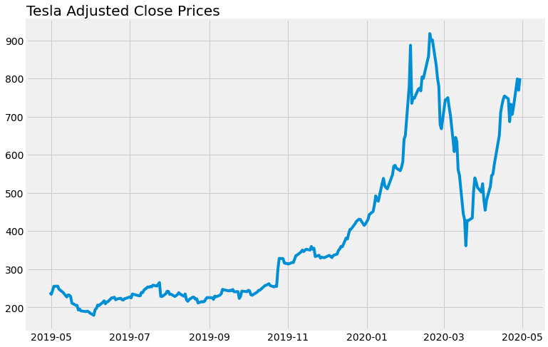
The dip in the price in March corresponds to the COVID-19 pandemic and the financial crisis that it brought with it.
It does seem to be on the rise now, so it will be interesting to see if the model can predict all these ups and downs.
Creating Series and Time arrays, and converting them to the right type:
series = np.array(adj_close.values)
time = np.array(dates)
series=pd.to_numeric(series,errors='coerce',downcast='float')
series
array([238.69, 234.01, 244.1 , 255.03, 255.34, 247.06, 244.84, 241.98,
       239.52, 227.01, 232.31, 231.95, 228.33, 211.03, 205.36, 205.08,
       192.73, 195.49, 190.63, 188.7 , 189.86, 188.22, 185.16, 178.97,
       193.6 , 196.59, 205.95, 204.5 , 212.88, 217.1 , 209.26, 213.91,
       214.92, 225.03, 224.74, 226.43, 219.62, 221.86, 223.64, 219.76,
       219.27, 222.84, 223.46, 227.17, 224.55, 234.9 , 233.1 , 230.34,
       230.06, 238.92, 238.6 , 245.08, 253.5 , 252.38, 254.86, 253.54,
       258.18, 255.68, 260.17, 264.88, 228.82, 228.04, 235.77, 242.26,
       241.61, 233.85, 234.34, 228.32, 230.75, 233.42, 238.3 , 235.01,
       229.01, 235.  , 219.62, 215.64, 219.94, 226.83, 225.86, 220.83,
       222.15, 211.4 , 215.  , 214.08, 215.59, 221.71, 225.61, 225.01,
       220.68, 229.58, 227.45, 231.79, 235.54, 247.1 , 245.87, 245.2 ,
       242.81, 244.79, 243.49, 246.6 , 240.62, 241.23, 223.21, 228.7 ,
       242.56, 242.13, 240.87, 244.69, 243.13, 233.03, 231.43, 237.72,
       240.05, 244.53, 244.74, 247.89, 256.96, 257.89, 259.75, 261.97,
       256.95, 253.5 , 255.58, 254.68, 299.68, 328.13, 327.71, 316.22,
       315.01, 314.92, 313.31, 317.47, 317.22, 326.58, 335.54, 337.14,
       345.09, 349.93, 346.11, 349.35, 352.17, 349.99, 359.52, 352.22,
       354.83, 333.04, 336.34, 328.92, 331.29, 329.94, 334.87, 336.2 ,
       333.03, 330.37, 335.89, 339.53, 348.84, 352.7 , 359.68, 358.39,
       381.5 , 378.99, 393.15, 404.04, 405.59, 419.22, 425.25, 430.94,
       430.38, 414.7 , 418.33, 430.26, 443.01, 451.54, 469.06, 492.14,
       481.34, 478.15, 524.86, 537.92, 518.5 , 513.49, 510.5 , 547.2 ,
       569.56, 572.2 , 564.82, 558.02, 566.9 , 580.99, 640.81, 650.57,
       780.  , 887.06, 734.7 , 748.96, 748.07, 771.28, 774.38, 767.29,
       804.  , 800.03, 858.4 , 917.42, 899.41, 901.  , 833.79, 799.91,
       778.8 , 679.  , 667.99, 743.62, 745.51, 749.5 , 724.54, 703.48,
       608.  , 645.33, 634.23, 560.55, 546.62, 445.07, 430.2 , 361.22,
       427.64, 427.53, 434.29, 505.  , 539.25, 528.16, 514.36, 502.13,
       524.  , 481.56, 454.47, 480.01, 516.24, 545.45, 548.84, 573.  ,
       650.95, 709.89, 729.83, 745.21, 753.89, 746.36, 686.72, 732.11,
       705.63, 725.15, 798.75, 769.12, 800.51], dtype=float32)
series.dtype
dtype('float32')
There are about 250 tuples, so a 80-20 split is somewhere around 210 for training set and 40 for testing set. The window size (for creating a windowed_dataset) and batch size can also be specified here.
split_time = 210
adj_train = series[:split_time]
adj_valid = series[split_time:]
dates_train=dates[:split_time]
dates_valid=dates[split_time:]

window_size = 16
batch_size = 32
shuffle_buffer_size = 50
A function for creating a windowed dataset can be specified here. This is particularly helpful because it helps to create specific sized data slices, to train on them, make predictions, and subsequently learn from those predictions as well.
def windowed_dataset(series, window_size, batch_size, shuffle_buffer):
    series = tf.expand_dims(series, axis=-1)
    ds = tf.data.Dataset.from_tensor_slices(series)
    ds = ds.window(window_size + 1, shift=1, drop_remainder=True)
    ds = ds.flat_map(lambda w: w.batch(window_size + 1))
    ds = ds.shuffle(shuffle_buffer)
    ds = ds.map(lambda w: (w[:-1], w[1:]))
    return ds.batch(batch_size).prefetch(1)
A function for forecasting data, given the series and the model can be specified here:
def model_forecast(model, series, window_size):
    ds = tf.data.Dataset.from_tensor_slices(series)
    ds = ds.window(window_size, shift=1, drop_remainder=True)
    ds = ds.flat_map(lambda w: w.batch(window_size))
    ds = ds.batch(32).prefetch(1)
    forecast = model.predict(ds)
    return forecast
Creating our windowed training set:
tf.keras.backend.clear_session()
tf.random.set_seed(51)
np.random.seed(51)
window_size = 64
batch_size = 256
train_set = windowed_dataset(adj_train, window_size, batch_size, shuffle_buffer_size)
print(train_set)
print(adj_train.shape)
<PrefetchDataset shapes: ((None, None, 1), (None, None, 1)), types: (tf.float32, tf.float32)>
(210,)
Specifying the layers of our Keras model.
It has 1 Convolutional Layer, which complements the windowing of the dataset. Simply through extensive trial and error, the configuration of 2 LSTMs (64 and 32 nodes), and 3 Dense Layers (24, 12 and 1 nodes) was selected here.
model = tf.keras.models.Sequential([
  tf.keras.layers.Conv1D(filters=60, kernel_size=5,
                      strides=1, padding="causal",
                      activation="relu",
                      input_shape=[None, 1]),
  tf.keras.layers.LSTM(64, return_sequences=True),
  tf.keras.layers.LSTM(32, return_sequences=True),
  tf.keras.layers.Dense(24, activation="relu"),
  tf.keras.layers.Dense(12, activation="relu"),
  tf.keras.layers.Dense(1),
  tf.keras.layers.Lambda(lambda x: x * 400)
])
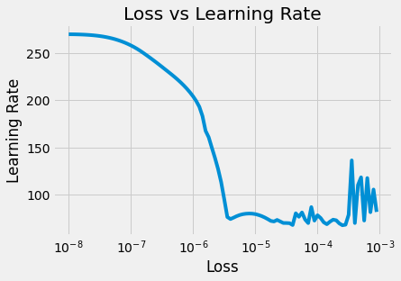
Before actually running our model in its entirity, it might help to specify a learning rate, so the model can be run for a specified number of epochs, and seeing how the model does, a optimized learning rate can be found. This hyperparameter tuning will prove to be very useful later.
lr_schedule = tf.keras.callbacks.LearningRateScheduler(
    lambda epoch: 1e-8 * 10**(epoch / 20))
optimizer = tf.keras.optimizers.SGD(lr=1e-8, momentum=0.9)
model.compile(loss=tf.keras.losses.Huber(),
              optimizer=optimizer,
              metrics=["mae"])
history = model.fit(train_set, epochs=100, callbacks=[lr_schedule])
Epoch 1/100
1/1 [==============================] - 0s 40ms/step - loss: 269.6010 - mae: 270.1010 - lr: 1.0000e-08
Epoch 2/100
1/1 [==============================] - 0s 2ms/step - loss: 269.5738 - mae: 270.0738 - lr: 1.1220e-08
Epoch 3/100
1/1 [==============================] - 0s 2ms/step - loss: 269.5186 - mae: 270.0186 - lr: 1.2589e-08
Epoch 4/100
1/1 [==============================] - 0s 2ms/step - loss: 269.4341 - mae: 269.9341 - lr: 1.4125e-08
Epoch 5/100
1/1 [==============================] - 0s 2ms/step - loss: 269.3180 - mae: 269.8180 - lr: 1.5849e-08
....
....
....
Epoch 96/100
1/1 [==============================] - 0s 2ms/step - loss: 72.6451 - mae: 73.1451 - lr: 5.6234e-04
Epoch 97/100
1/1 [==============================] - 0s 2ms/step - loss: 117.5780 - mae: 118.0779 - lr: 6.3096e-04
Epoch 98/100
1/1 [==============================] - 0s 2ms/step - loss: 81.4628 - mae: 81.9628 - lr: 7.0795e-04
Epoch 99/100
1/1 [==============================] - 0s 2ms/step - loss: 105.4503 - mae: 105.9502 - lr: 7.9433e-04
Epoch 100/100
1/1 [==============================] - 0s 2ms/step - loss: 81.7803 - mae: 82.2790 - lr: 8.9125e-04
Plotting the results of the limited run of the model:
plt.title("Loss vs Learning Rate")
plt.xlabel("Loss")
plt.ylabel("Learning Rate")
plt.semilogx(history.history["lr"], history.history["loss"])
#plt.axis([1e-8, 1e-3,135,250])
[<matplotlib.lines.Line2D at 0x7f3e82620048>]
tf.keras.backend.clear_session()
tf.random.set_seed(51)
np.random.seed(51)
model = tf.keras.models.Sequential([
  tf.keras.layers.Conv1D(filters=60, kernel_size=5,
                      strides=1, padding="causal",
                      activation="relu",
                      input_shape=[None, 1]),
  tf.keras.layers.LSTM(256, return_sequences=True),
  tf.keras.layers.LSTM(128, return_sequences=True),
  tf.keras.layers.Dense(128, activation="relu"),
  tf.keras.layers.Dense(64, activation="relu"),
  tf.keras.layers.Dense(1),
  tf.keras.layers.Lambda(lambda x: x * 500)
])


optimizer = tf.keras.optimizers.SGD(lr=3e-7, momentum=0.9)
model.compile(loss=tf.keras.losses.Huber(),
              optimizer=optimizer,
              metrics=["mae"])
history = model.fit(train_set,epochs=350)
Epoch 1/350
1/1 [==============================] - 0s 7ms/step - loss: 330.9964 - mae: 331.4964
Epoch 2/350
1/1 [==============================] - 0s 901us/step - loss: 314.5646 - mae: 315.0646
Epoch 3/350
1/1 [==============================] - 0s 849us/step - loss: 295.7275 - mae: 296.2275
Epoch 4/350
1/1 [==============================] - 0s 986us/step - loss: 277.2317 - mae: 277.7317
Epoch 5/350
1/1 [==============================] - 0s 835us/step - loss: 244.2985 - mae: 244.7985
Epoch 6/350
1/1 [==============================] - 0s 860us/step - loss: 225.8815 - mae: 226.3815
Epoch 7/350
1/1 [==============================] - 0s 836us/step - loss: 208.5272 - mae: 209.0272
Epoch 8/350
1/1 [==============================] - 0s 2ms/step - loss: 184.0172 - mae: 184.5172
Epoch 9/350
1/1 [==============================] - 0s 895us/step - loss: 158.5788 - mae: 159.0788
Epoch 10/350
1/1 [==============================] - 0s 988us/step - loss: 140.6364 - mae: 141.1363
...
...
...
Epoch 101/350
1/1 [==============================] - 0s 927us/step - loss: 48.9045 - mae: 49.4025
Epoch 102/350
1/1 [==============================] - 0s 833us/step - loss: 47.7830 - mae: 48.2795
Epoch 103/350
1/1 [==============================] - 0s 844us/step - loss: 47.8659 - mae: 48.3605
Epoch 104/350
1/1 [==============================] - 0s 1ms/step - loss: 48.0967 - mae: 48.5908
Epoch 105/350
1/1 [==============================] - 0s 832us/step - loss: 46.6607 - mae: 47.1546
...
...
...
Epoch 200/350
1/1 [==============================] - 0s 2ms/step - loss: 25.1572 - mae: 25.6457
Epoch 201/350
1/1 [==============================] - 0s 842us/step - loss: 25.0279 - mae: 25.5159
Epoch 202/350
1/1 [==============================] - 0s 1ms/step - loss: 25.0110 - mae: 25.4993
Epoch 203/350
1/1 [==============================] - 0s 889us/step - loss: 24.9164 - mae: 25.4044
Epoch 204/350
1/1 [==============================] - 0s 933us/step - loss: 24.9017 - mae: 25.3895
Epoch 205/350
1/1 [==============================] - 0s 1ms/step - loss: 24.7882 - mae: 25.2767
...
...
...
Epoch 300/350
1/1 [==============================] - 0s 1ms/step - loss: 22.3528 - mae: 22.8462
Epoch 301/350
1/1 [==============================] - 0s 844us/step - loss: 20.8384 - mae: 21.3259
Epoch 302/350
1/1 [==============================] - 0s 779us/step - loss: 19.6541 - mae: 20.1386
Epoch 303/350
1/1 [==============================] - 0s 820us/step - loss: 19.2455 - mae: 19.7316
Epoch 304/350
1/1 [==============================] - 0s 1ms/step - loss: 19.0995 - mae: 19.5838
Epoch 305/350
1/1 [==============================] - 0s 922us/step - loss: 19.0408 - mae: 19.5255
...
...
...
Epoch 345/350
1/1 [==============================] - 0s 914us/step - loss: 19.7900 - mae: 20.2793
Epoch 346/350
1/1 [==============================] - 0s 836us/step - loss: 18.8462 - mae: 19.3341
Epoch 347/350
1/1 [==============================] - 0s 963us/step - loss: 18.4283 - mae: 18.9135
Epoch 348/350
1/1 [==============================] - 0s 852us/step - loss: 18.3297 - mae: 18.8162
Epoch 349/350
1/1 [==============================] - 0s 963us/step - loss: 18.4796 - mae: 18.9658
Epoch 350/350
1/1 [==============================] - 0s 1ms/step - loss: 19.0140 - mae: 19.5016
The MAE (Mean Absolute Error) seems pretty low after running it for 350 epochs, which is an excellent sign. It started at ~330 and ended around ~19. Now we can build a forecast using the model_forecast function specified earlier:
rnn_forecast = model_forecast(model, series[..., np.newaxis], window_size)
rnn_forecast = rnn_forecast[split_time - window_size:-1,-1, 0]
There are mainly 2 metrics used for evaluating the accuracy of time series data, Mean Absolute Error and Root Mean Squared Error.
n = tf.keras.metrics.MeanAbsoluteError()
n.update_state(adj_valid, rnn_forecast)
print('Mean Absolute Error: ', n.result().numpy())
m = tf.keras.metrics.RootMeanSquaredError()
m.update_state(adj_valid, rnn_forecast)
print('Root Mean Squared Error: ', m.result().numpy())
Mean Absolute Error:  152.27446
Root Mean Squared Error:  171.10997
Considering the fact that there was only 250 data points, and a pretty simple RNN built, a MAE of 150 and RMSE of 171 is extremely good. With more data, and a bigger model, it’s very possible to reduce these numbers.
Plotting the predicted data against what actually happened:
plt.figure(figsize=(20, 6))
plt.style.use('fivethirtyeight')
plt.title("Predictions vs Reality", loc="left")
plt.plot(dates_valid, adj_valid, label="Actual")
plt.plot(dates_valid, rnn_forecast, label= "Prediction")
plt.legend()
<matplotlib.legend.Legend at 0x7f12360679e8>
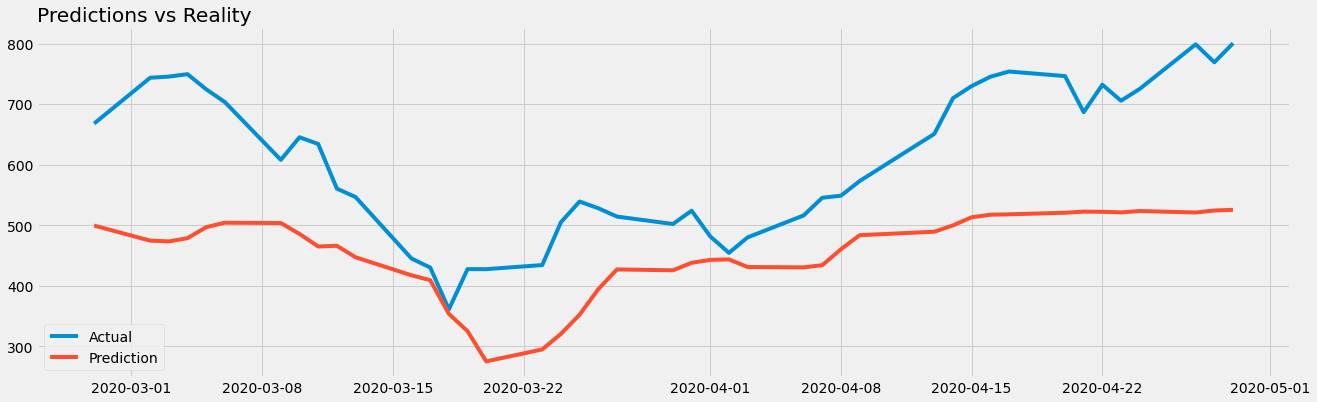
The model seemed to have gotten it pretty spot-on. It dips when the actual value dipped and seems to be on the rise, as is the case towards the end.